Signal Processing

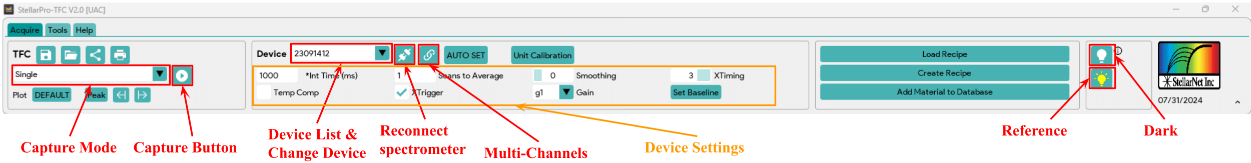
1. Make sure your spectrometer is plugged in connected. If not, left-click on the “Reconnect spectrometer” button to make a connection between the program and your spectrometer. A prompt will appear alerting to a successful connection. The serial number of the spectrometer will help to indicate which instrument is being connected.
   
2. After the spectrometer is connected, click the “Capture” button once to collect one scan. The data collection panel will default to “Single” – do not use Loop or Episodic unless it is necessary for your application.
3. Align the reflectance probe with the reference sample. Typically, the optimal reference sample is the substrate without any coatings. Turn ON the light source.
4. Next, optimize the reference curve and adjust the signal-to-noise ratio of the spectrometer. Enter the desired time in the integration time input box, then click on the “Int Time (ms)” button next to the input textbox to apply the entered time. The goal is to maximize your signal in SCOPE mode with the reference sample and light source turned ON. You want to adjust your integration time until the spectrum fills most of the SCOPE graph (65,000) without saturating. This is also the point at which you should adjust the number of scans to average (more scans averaged will increase accuracy, but will take more time for each reading). You can also add smoothing controls at this time in the Device Settings block. A pixel box car set to 3 and averaging set to 5 often gives nice results. 
   

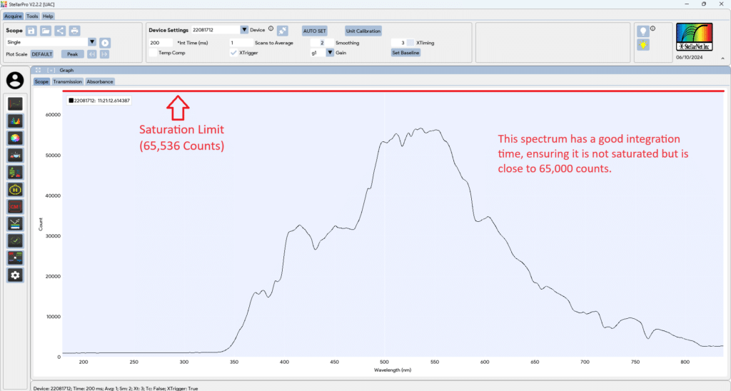
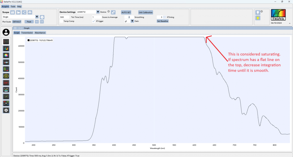
   In the first picture below, the spectrum is correctly optimized to be just below the saturation limit (65,536 counts). In the second picture below, the spectrum have a flat line on the top, indicating the need to reduce the integration time.

5. Now, it is time to take references. Turn OFF the lamp and left click on the dark bulb . The baseline will subtract out and flatten at the bottom of the Scope mode graph. The subtracted spectrum will be counted as 0% transmission/reflectance for future calculations, until overwritten.
   • Note: A right-click will release the dark bulb– this is often recommended to do before optimizing settings (Integration Time, Smoothing, Scans to Average).
   • Note: Hovering the mouse pointer over the icon will pull up a tool-tip indicating if the dark reference has been captured.
6. Turn ON the lamp, make sure that the reference standard is in proper geometrical position and left-click on the “Reference” icon . This will set the upper boundary for transmission/reflectance measurement and count the spectrum as 100% for future calculations, until overwritten.
7. The upper left-hand corner has selectable tabs for the raw Scope mode display and the Reflectance mode display. The bottom left-hand corner displays the serial number of the device being used, integration time (1-65536), scan averaging (1-1000), pixel-boxcar smoothing (0-4), X-timing resolution control (should always be set to 3), temperature compensation (set to off unless operating in an environment with temperature drifts), and triggering timeout (on/off).
8. Click on Reflectance tab in the Graph window to view the reflectance plot. There will be noise in regions where there is little signal to noise due to a lack of light signal in the raw Scope data.
9. To combat the noise, the user can increase the integration time even further to try to get closer to the saturation point without saturating. The closer the signal gets to the saturation point, the higher risk that the detector saturates. This is not a damage concern as much as it is a concern of data. The recommended setting is to be at ~90% of the maximum.
10. If the noise is present in the UV region and the spectrometer is capable of detecting signals in the UV range, a Deuterium lamp is recommended. StellarNet offers the SL1-SL3 Combo, SL3, and SL4 lamps for UV reflectance applications. The SL5-DH deuterium halogen lamp is only appropriate for transmission applications. If the noise is present in the NIR region, a halogen lamp should be used and it may become necessary to use an InGaAs detector for the 900-1700nm range or Extended InGaAs for 900-2500nm range as Si-CCD and CMOS detectors have limited sensitivity in the 900-1100nm range. Another way to stabilize data is to increase sample averaging, and increase smoothing of the data.
11. Now that settings have been configured, signal has been optimized, and references have been taken, it is time to perform some measurements.
12. Before a measurement is taken, a recipe must be loaded. Before a recipe can be loaded, a recipe must be created. Review the following Recipe Creation and Performing a Measurement sections.